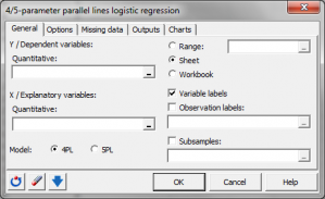
Four/Five-parameter parallel lines logistic regression

What is four/five-parameter parallel lines logistic regression?

Four parameter logistic model

The four parameter logistic model writes:

y = a + (d -a) / [1 + (x / c)^b] model (1.1)

where a, b, c, d are the parameters of the model, and where x corresponds to the explanatory variable and y to the response variable. a and d are parameters that respectively represent the lower and upper asymptotes, and b is the slope parameter. c is the abscissa of the mid-height point which ordinate is (a+b)/2. When a is lower than d, the curve decreases from d to a, and when a is greater than d, the curve increases from a to d.

Five parameter logistic model

The five parameter logistic model writes:

y = a + (d -a) / [1 + (x / c)^b]^e model (1.2)

where e is an additional parameter, the asymmetry factor.

Four parameter parallel lines logistic model

The four parameter parallel lines logistic model writes:

y = a + (d -a) / [1 + (s0 * x / c₀ + s1 * x / c₁)^b] model (2.1)

where s0 is 1 if the observation comes from the standard sample, and 0 if not, and where s1 is 1 if the observation is from the sample of interest, and 0 if not. This is a constrained model because the observations corresponding to the standard sample influence the optimization of the values of a, b, and d. From the above writing of the model, one can understand that this model generates two parallel curves, which only difference is the positioning of the curve, the shift being given by (c1-c0). If c1 is greater than c0, the curve corresponding to the sample of interest is shifted to the right of the curve corresponding to the standard sample, and vice-versa.)

Five parameter parallel lines logistic model

The five parameter parallel lines logistic model writes:

y = a + (d -a) / [1 + (st * x / c₀ + sp * x / c₁)^b]^e model (2.2)

What XLSTAT can do

XLSTAT allows to fit:

•    model 1.1 or 1.2 to a standard sample or to the sample of interest,
•    model 2.1 or 2.2 to the standard sample and and to the standard sample the same time.

XLSTAT allows to either fit models 1.1 or 1.2 to a given sample (A case), or to fit models 1.1 or 1.2 to the standard (0) sample and then fit models 2.1 or 2.2 to both the standard sample and the sample of interest (B case).
If the Dixon’s test option is activated, XLSTAT tests for each sample if some outliers influence too much the fit of the model. In the A case, a Dixon’s test is performed once the model 1.1 or 1.2 is fitted. If an outlier is detected, it is removed, and the model is fitted again, and so on, until no outlier is detected. In the B case, we first perform a Dixon’s test on the standard sample, then on the sample of interest, and then, the models 2.1 or 2.2 is fitted on the merged samples, without the outliers.
In the B case, and if the sum of the sample sizes is greater than 9, a Fisher’s F test is performed to detect if the a, b, d and e parameters obtained with models 1.1 or 1.2 are not significantly different from those obtained with model 2.1 or 2.2.

Results displayed by XLSTAT

If no group or a single sample was selected, the results are shown for the model and for this sample. If several sub-samples were defined (see sub-samples option in the dialog), the model is first adjusted to the standard sample, then each sub-sample is compared to the standard sample.

Fisher's test assessing parallelism between curves: The Fisher’s F test is used to determine if one can consider that the models corresponding the standard sample and the sample of interest are significantly different or not. If the probability corresponding to the F value is lower than the significance level, then one can consider that the difference is significant.
Goodness of fit coefficients: This table shows the following statistics:
•    The number of observations;
•    The number of degrees of freedom (DF);
•    The determination coefficient R2;
•    The sum of squares of the errors (or residuals) of the model (SSE or SSR respectively);
•    The means of the squares of the errors (or residuals) of the model (MSE or MSR);
•    The root mean squares of the errors (or residuals) of the model (RMSE or RMSR);

Model parameters: This table displays the estimator and the standard error of the estimator for each parameter of the model. It is followed by the equation of the model.
Predictions and residuals: This table displays giving for each observation the input data and corresponding prediction and residual. The outliers detected by the Dixon’s test, if any, are displayed in bold.

Charts: On the first chart are displayed in blue color, the data and the curve corresponding to the standard sample, and in red color, the data and the curve corresponding to the sample of interest. A chart that allows to compare predictions and observed values as well as the bar chart of the residuals are also displayed.