Heteroscedasticity tests

What is heteroscedasticity?

The concept of heteroscedasticity - the opposite being homoscedasticity - is used in statistics, especially in the context of linear regression or for time series analysis, to describe the case where the variance of errors of the model is not the same for all observations, while often one of the basic assumption in modeling is that the variances are homogeneous and that the errors of the model are identically distributed.

Why is heteroscedasticity a problem? In linear regression analysis, the fact that the errors of the model (also named residuals) are not homoskedastic has the consequence that the model coefficients estimated using ordinary least squares (OLS) are neither unbiased nor those with minimum variance. The estimation of their variance is not reliable.

How to check for Heteroscedasticity in XLSTAT

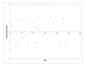
If it is suspected that the variances are not homogeneous (a representation of the residuals against the explanatory variables may reveal heteroscedasticity), it is therefore necessary to perform a test for heteroscedasticity. Several tests have been developed, with the following null and alternative hypotheses:

• H0 : The residuals are homoscedastic
• Ha : The residuals are heteroscedastic

Breusch-Pagan test

This heteroscedastiicity test has been developed by Breusch and Pagan (1979), and later improved by Koenker (1981) - which is why this test is sometimes named the Breusch- Pagan and Koenker test - to allow identifying cases of heteroscedasticity, which make the classical estimators of the parameters of the linear regression unreliable. If e is the vector of the errors of the model, the null hypothesis H0 of said error terms being of constant variance can write:

H₀ : E(e²) = σ²

To verify that the quadratic errors are independent of the explanatory variables, which can translate into many functional forms, the simplest is to regress the squared errors by the explanatory variables. If the data are homoskedastic, the coefficient of determination R² should then not be equal to 0. If H0 is not rejected we can conclude that heteroscedasticity, if it exists, does not take the functional form used. Practice shows that heteroscedasticity is not a problem if H0 is not accepted. If H0 is rejected, it is likely that there is heteroscedasticity and that it takes the functional form described above.

The statistic used for the test, proposed by Koenker (1981) is:

LM = nR²

where LM stands for Lagrange multiplier. This statistic has the advantage of asymptotically following a Chi-square distribution with p degrees of freedom, where p is the number of explanatory variables.

If the null hypothesis is rejected, it will be necessary to transform the data before doing the regression, or using modeling methods to take into account the variability of the variance.

White test and modified White test(Wooldridge)

How to detect heteroscedasticity using White test? This test was developed by White (1980) to identify cases of heteroscedasticity making classical estimators of the parameters of linear regression unreliable. The idea is similar to that of Breusch and Pagan, but it relies on weaker assumptions as for the form that heteroscedasticity takes. This results in a regression of the quadratic errors by the explanatory variables and by the squares and cross-products of the latter. The statistic used is the same as the test-Breusch Pagan, but due to the presence of many more regressors, there are here 2p+p*(p-1)/2 degrees of freedom for the Chi-square distribution.

In order to avoid losing too many degrees of freedom, Wooldrigde (2009) proposed to regress the squared errors by the model predictions and by their square. This reduces to 2 the number of degrees of freedom for the Chi-square.

How to fix heteroscedasticity in XLSTAT

Newey West and other estimators 

XLSTAT allows you to apply corrections for heteroscedasticity. Several estimators (Newey West, HC0, HC1, etc) for this purpose are available in the Linear Regression tool.

White (1980) followed by several authors has explored ways to correct the classical estimate of the covariances using residuals and centered leverages obtained from the linear regression computations (see MacKinnon (1985) and Zeileis (2006) for a review). When the assumptions of classical linear regression do not hold, while the estimators of the coefficients are unchanged, the simplified writing of the covariance matrix of the beta parameters is not possible, and we must revert to the general expression:

Var (β) = (X^tX)^-1 (X^t ΩX)(X^tX)^-1

Transformation of the dependent variable

You may use the XLSTAT variables transformation tool to apply a Box-Cox transformation in order to correct heteroscedasticity.

Weighted regression

You may also fit a weighted regression to deal with heteroscedasticity. Every regression model in XLSTAT allows us to select weights through its dialog box. 

Results for heteroscedasticity tests in XLSTAT 

The output includes:

• a summary statistics table 
• a residuals plot
• the results of the selected tests (statistic of the test, critical value, p-value, alpha)

Tutorial on Heteroscedasticity tests

Wondering how to run a heteroscedasticity test in Excel? Read about how to set up and interpret an heteroscedasticity test in Excel using the XLSTAT software.